Partial Fraction Decomposition | ||
|
Introduction | |
This lesson page will teach you how to take a complicated rational expression and transform it into the sum or difference of less complicated rational expressions. Here are the sections within this lesson page:
| |
Before continuing with this lesson, it is necessary to have background knowledge within several mathematics topics. Those topics are listed below. If you are not familiar with them or if you find that you are having difficulty understanding this lesson, please review them before continuing.
| |
Take a look at this rational expression:

Let us examine the numerator.

The numerator is a linear expression, which means it is a degree one binomial. Here is the denominator.

The denominator is degree two. It can also be factored.

This means the original rational expression could be written as this.

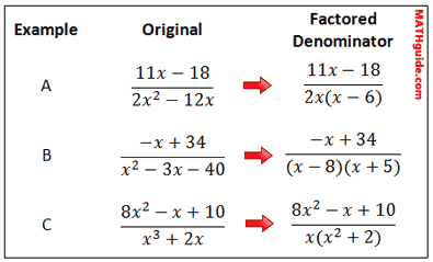
Here are several other rational expressions and their factored (denominator) forms.

Use our lesson on Rational Expressions to review how it is we add, subtract, and multiply rational expressions.
| |
When we decompose rational expressions by transforming them from the complex to sums and differences of simpler rational expressions, we have to work with factored denominators. The process involves using those factored denominators and writing them within new rational expressions.

The factored form is �

The decomposition process tells us to create a fraction for each variable factor in the denominator, like so.

To determine the numerators, we have to write expressions that are of one less degree than their respective denominators. Both denominators are degree one, so we will write the numerators with degree zero expressions.

This problem has now been rewritten as less complicated rational expressions. This is the beginning of the process and we will explore the complete process within our next section.
Example B:

We will now write the rational expression as a sum of less complicated rational expressions.

The beginning step is done. Now, to our last example...
Example C:

Here it is with a factored denominator.

Now, we will break up the rational expression into less complicated fractions, like so.

Notice how the second denominator of the right side of the equation contains a degree two polynomial. Consequently, a polynomial of one less degree was written in the numerator.
The next section will take the process to the conclusion. We will determine how to calculate for the polynomial expressions that were created in the numerators.
| |
Within the last section, we learned how to start the process using Decomposition Examples. In this section, we will carry two problems all the way through to the end.

To solve for the A-value and the B-value, we need to gain a common denominator. So, we will multiply the fractions until each denominator matches the denominator of the original fraction.

We need to multiply the fractions.

Now, we combine fractions and arrange like terms.

Since the denominators are equal, we only need to concern ourselves with the numerators.

For two polynomials to be equal to each other, their corresponding coefficients must also be equal. This gives us two equations. Here is the first, by examining the x-terms.

The next equation comes from looking at the constant term.

So this is the system of equations we must solve.

Clearly, the second equation can be solved for A. The A-value is equal to 3. Substituting that value into the first equation, we get the B-value. The B-value is 4. Since the A-value is 3 and the B-value is 4, these values can be substituted into the format of our partial fraction decomposition, which renders this.

We are done with this example. We also have a video that explains how to do this.
Here is another example.
Example C:

We will work through this problem more quickly. First, we need a common denominator.

Now, let us multiply the fractions.

With a common denominator on the right hand side of the equation, we get this.

Looking at the coefficients of the x-squared terms, we get this equation.

Looking at the coefficients of the x-terms, we get this equation.

Looking at the constant terms, we get this equation.

This leads us to a system of equations.

The third equation gives us the A-value, which is 5. Using that value within the first equation, we get the B-value, which is 3. Now, we can use these values within our partial fraction decomposition setup, like so.

| |
Watch this video on partial fraction decomposition. | |
Try our interactive quizzes to determine if you understand the lessons above. | |
Try these lessons, which are closely related to the lessons above.
| |
 esson:
  ideo:
ideo:  uiz:
uiz: